Authors: Aaron Chester, Ron Fox, Jeromy Tompkins

Date: 4/3/24

Introduction

: This document describes the simplest DDAS setup: A single PXI crate with one digitizer. Throughout, there will be suggestions on how to expand this setup so that it has several digitizers. This material is organized as follows:

First, an overview of the components of a single crate DDAS system are given.
Second, we provide a guide to setting up the hardware. A pulser will be used as a signal source.
The configuration files for the system and expected event length required by DDAS are described.
QtScope will be used to obtain an initial parameter setup.
We will set up a readout so that data can be taken from the sample setup. We'll also look at a dump of the data from the simple setup with and without waveforms.
We'll show how to set up the ReadoutGUI and event builder so that data can be taken, built into events, recorded, and made available for online analysis.
We will set up a simple SpecTcl tailoring for data with and without waveforms.
We will import the data into ROOT so that offline analysis can proceed with that tool.

Attention

This single-crate system setup guide is specific to DDAS systems running NSCLDAQ 12 and later, which has a handful of major features which were not part of previous releases:

The module data readout and sorting processes are decoupled. As a consequence, readout program data sources must be configured in a slightly different manner.
The DDAS codebase has been refactored into NSCLDAQ, there is no need to source a DDAS setup script in e.g., /usr/opt/ddas.
External clock readout has been absorbed into the main readout program. There is no longer a separate version of the DDAS readout for this purpose.
As of XIA API major version 3, settings files are saved in JSON format. Files with names like crate_1.json are the JSON version of the binary settings files generally named crate_1.set for previous XIA API releases. Note that there is no strict enforcement of file extensions: a JSON settings file can be saved with a .set extension. The .json extension is used here to remind the reader familiar with older versions of the NSCLDAQ that these settings files are not the binary settings files they are familiar with. Further it should be noted that JSON settings file are not back-compatible with older NSCLDAQ versions using XIA API 2, and that there is no supported way to convert a JSON settings file into binary format.

Components of a DDAS System

: DDAS data acquisition systems and online analysis rely on several hardware and software components:

A PXI Crate. PXI is an extension to the compact PCI standard that supports precision timing.
One or more XIA digitizer cards.
An interface between an NSCL spdaq system and the PXI crate or a crate-resident single-board computer (SBC). These two options will be referred to as the data-collection computer.
A readout program that runs in the data-collection computer that reads data from the digitizer cards and places them into a raw ringbuffer. This readout program is the interface between the PXI crate and the NSCLDAQ software.
A sorter program which reads data from a raw ringbuffer, maintains a master list of sorted hits, and outputs those hits into a sorted ringbuffer for event building.
An event builder. The event builder takes data from sorted ringbuffers, builds events that satisfy a coincidence interval using the DDAS timestamp and places those built events in an output ringbuffer. Note that while in principle the event builder is not necessary for single-crate systems, using it for those systems maintains a common event format between single- and multi-crate systems.
A ReadoutShell instance that manages readout, sorting, event logging and event building.
A SpecTcl tailored to decode DDAS data and analyze it in an experiment-specific manner.

: The following figure shows a schematic representation of a DDAS hardware configuration using one crate:

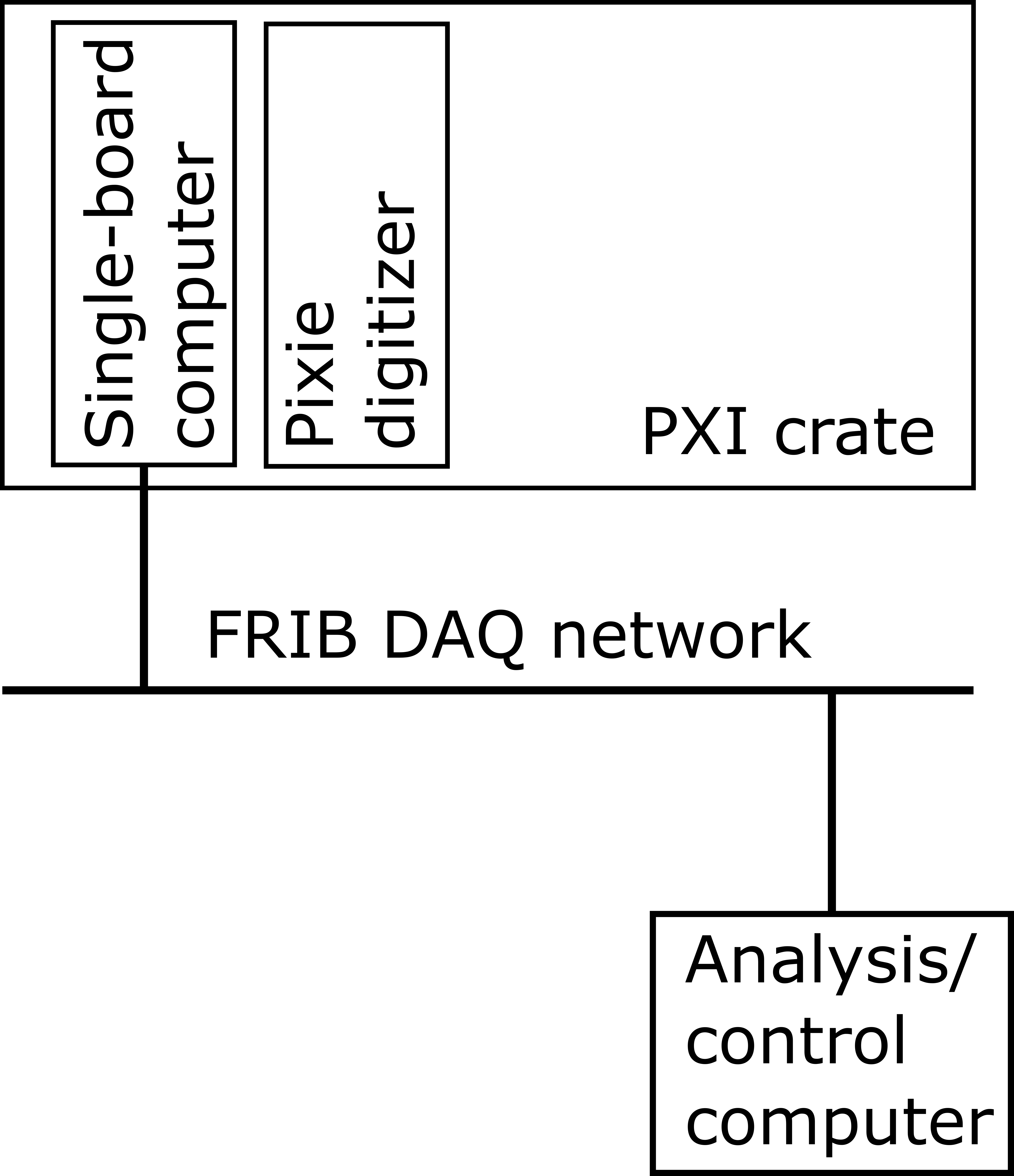
A schematic DDAS hardware configuration. A PXI crate with an SBC used as the data-collection computer and a single Pixie module is connected via the FRIB DAQ network to an analysis computer.

: The data flow through such a system looks like:

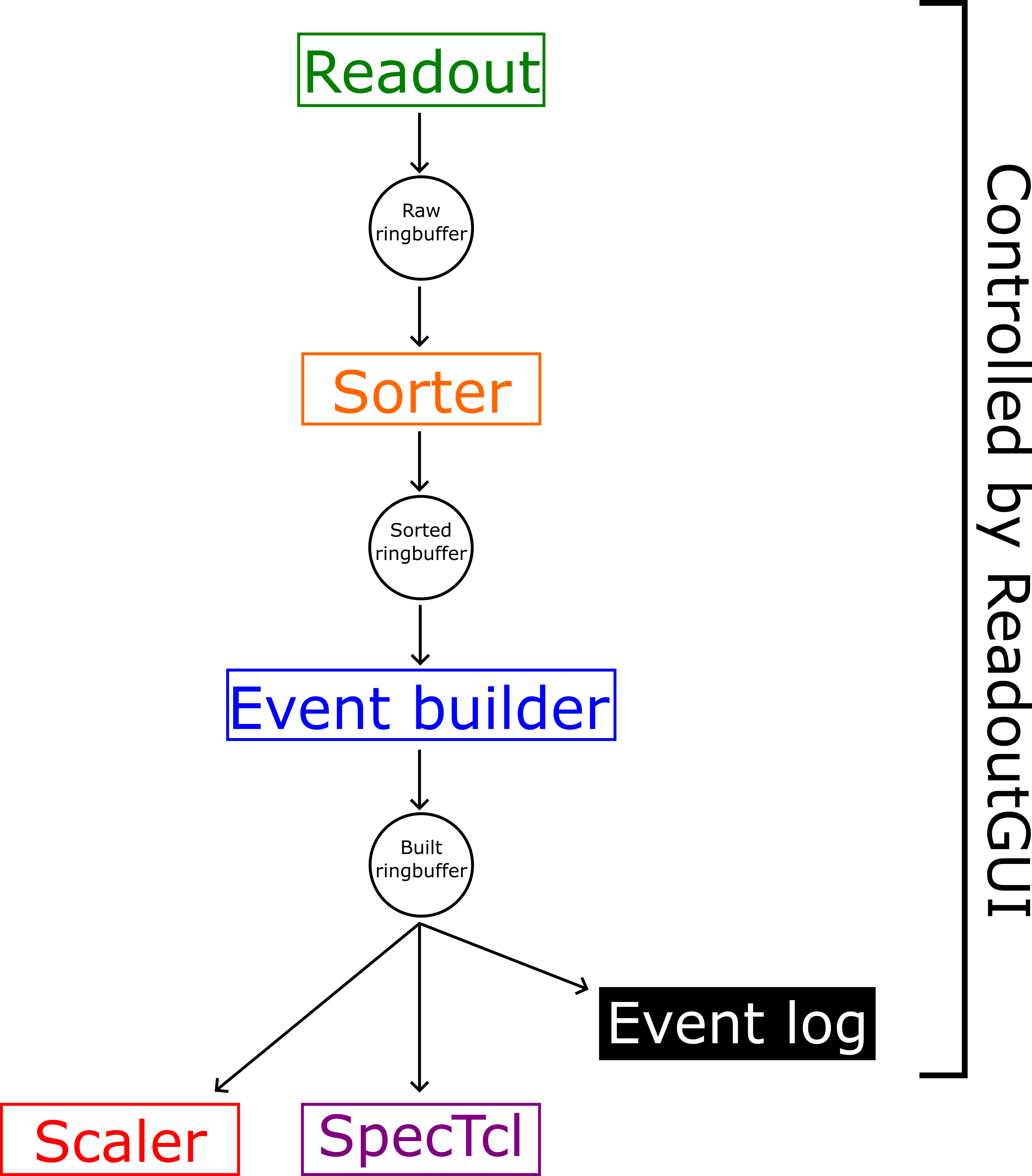
Data flow through a DDAS system running NSCLDAQ 12. Note the separation of module data readout and sorting, which were previously part of a single process. This configuration enables much higher data readout speeds.

A couple of points are worth noting:

The analysis computer is not strictly necessary. All of the software can be run on the data-collection computer.
In the usual production configuration (i.e. during an experiment) the only program that will run on the data-collection computer is the readout program. All other pieces of the software shown on the above figure will run other places.
For multi-crate systems, the schematics can be expanded by adding additional crates to the hardware diagram and additional readout and sort paths feeding the event builder to the data flow diagram.
Adding additional digitizers to an already-configured system is (mostly) just a matter of editing the system configuration files.

Getting Started

: The DDAS software is installed as part of the NSCLDAQ software package. There may be several versions of NSCLDAQ installed concurrently on lab computers. In general these will be located under /usr/opt/daq on FRIB computer systems. Each NSCLDAQ installation has a version number MM.mm-eee where MM refers to the major version, mm to the minor version, and eee to an edit level e.g. 12.0-017 with major version 12, minor version 0, and edit level 15. Edit-level changes reflect minor defect fixes or enhancements, minor-version changes reflect more impactful bug fixes or enhancements. Major version changes are generally quite significant and may require significant rewrites of user code.

Each NSCLDAQ version's top-level directory includes a daqsetup.bash script which can be sourced to set the following environment variables:

DAQROOT- Points to the top-level NSCLDAQ installation directory (containing the daqsetup.bash script.
DAQBIN - Points to $DAQROOT/bin, the directory containing NSCLDAQ executables.
DAQLIB - Points to $DAQROOT/lib, the directory containing NSCLDAQ libraries which DDAS applications and user code may need to link against.
DAQINC - Points to $DAQROOT/include, the directory containing NSCLDAQ header files including those for DDAS.
DAQSHARE - Points to $DAQROOT/share, a directory containing documentation, program skeletons, and scripts.

Loading the PLX Kernel Driver

: Users are no longer required to load the PLX kernel module by hand on each data-readout computer installed as part of your DDAS system. The kernel module is loaded automatically on system startup.

Configuration Files Needed by NSCL DDAS

: Many of the DDAS software components require a set of configuration files to be in the current working directory. These configuration files describe the configuration of modules in a crate and point at a settings file containing the parameters used by the digital signal-processing (DSP) algorithms for each module in use. By convention a directory sub-tree is used to hold the configuration files for each crate. The tree will look something like:

home-directory
      |
      +--- readout
              |
              +--- crate_1  (configuration for crate 1)
              +--- crate_2  (configuration for crate 2, if needed)
              ...
              +--- crate_n  (configuration for crate n, if needed)

: We can expand the full directory tree for a single-crate system:

home-directory
     |
     +-- readout
            |
            +--- crate_1
                    |
                    +--- cfgPixie16.txt
                    +--- modevtlen.txt
                    +--- crate_1.json

An example crate_1 directory which can be copied to your system can be found at $DAQSHARE/ddasreadout/crate_1. This example directory contains the necessary configuration files to run a DDAS system. The files are:

cfgPixie16.txt - Indicates where modules are installed in the crates and points to a parameter settings file containing their DSP settings. See the documentation for this file here.
modevtlen.txt - Describes the number of 32-bit words in a hit for each module. See the documentation for this file here.
crate_1.json - An XIA API 4 parameter settings file.

: See the documentation for the cfgPixie16.txt and modevtlen.txt files for more information.

Note

While $DAQSHARE/ddasreadout/crate_1 contains a valid set of configuration files for DDAS, there is no guarantee that the configuration files or settings file in the example directory are correct for any given system. You will may need to edit all of these files in order to get your system running correctly. Typical changes are:

cfgPixie16.txt must be modified to reflect the layout of modules in your crate. The path to the settings file must be correct.
The name of the settings file must match that within the cfgPixie16.txt file.
modevtlen.txt must be modified to reflect your actual event sizes if extra data words from e.g., QDC sums or trace data are expected.

Setting Up a Single-Crate System

This part of the guide will discuss in detail how to setup a single-crate DDAS system with a single XIA digitizer card. You must:

Ensure that there is an SBC or fiber interface in slot 1 of the PXI crate (the most common case). If a fiber interface is used, the fiber must be connected to the interface card and a PCI bridge card on the data-collection computer. The data-collection computer must be connected to the DAQ network.
Install a Pixie module configured as a clock master in slot 2 of your crate.
Attach signals to the digitizer inputs. One of the nice things about digital data acquisition modules is that only minimal signal conditioning is required and the modules themselves handle triggering. For this tutorial we're going to take singles data. The modules actually support very sophisticated internal triggering modes as well as cross-module trigger processing via a front-panel trigger bus.
Configure your DSP settings.

Attention: At FRIB, the NSCLDAQ software is run from within a container. To run the NSCLDAQ software discussed in this tutorial, you may need to edit your container startup script or script(s) you use to launch NSCLDAQ programs following the instructions provided under "Containerized NSCLDAQ" found on the SDAQ homepage. For systems running Singularity, you must define the environment variable SING_IMAGE to be the full image path and store the bindings you are using in the ~/.singularity_bindpoints file.

: Step 1 is relatively straightforward and need not be discussed further. Steps 2-4 are more complex and will be covered in detail in the subsequent sections.

Warning: SBCs, fiber cards and modules are NOT hot-swappable. DO NOT connect or disconnect SBCs, fiber cards or modules from the crate while it is powered on. Before installing or replacing any DDAS hardware, ensure that the crate is powered off.

Clock Distribution Settings for a Single-Crate System

: When using several DDAS cards it is important to synchronize the digitizer clocks between them. This is done by setting the jumper block JP01 appropriately. The jumper block is a set of pins located on the board near the backplane connectors, shown on the figure below in the red box. Configure the connections between these pins with jumpers. In case your setup consists of a single module, be sure to configure the jumpers to match the top diagram for the PXI clock master.

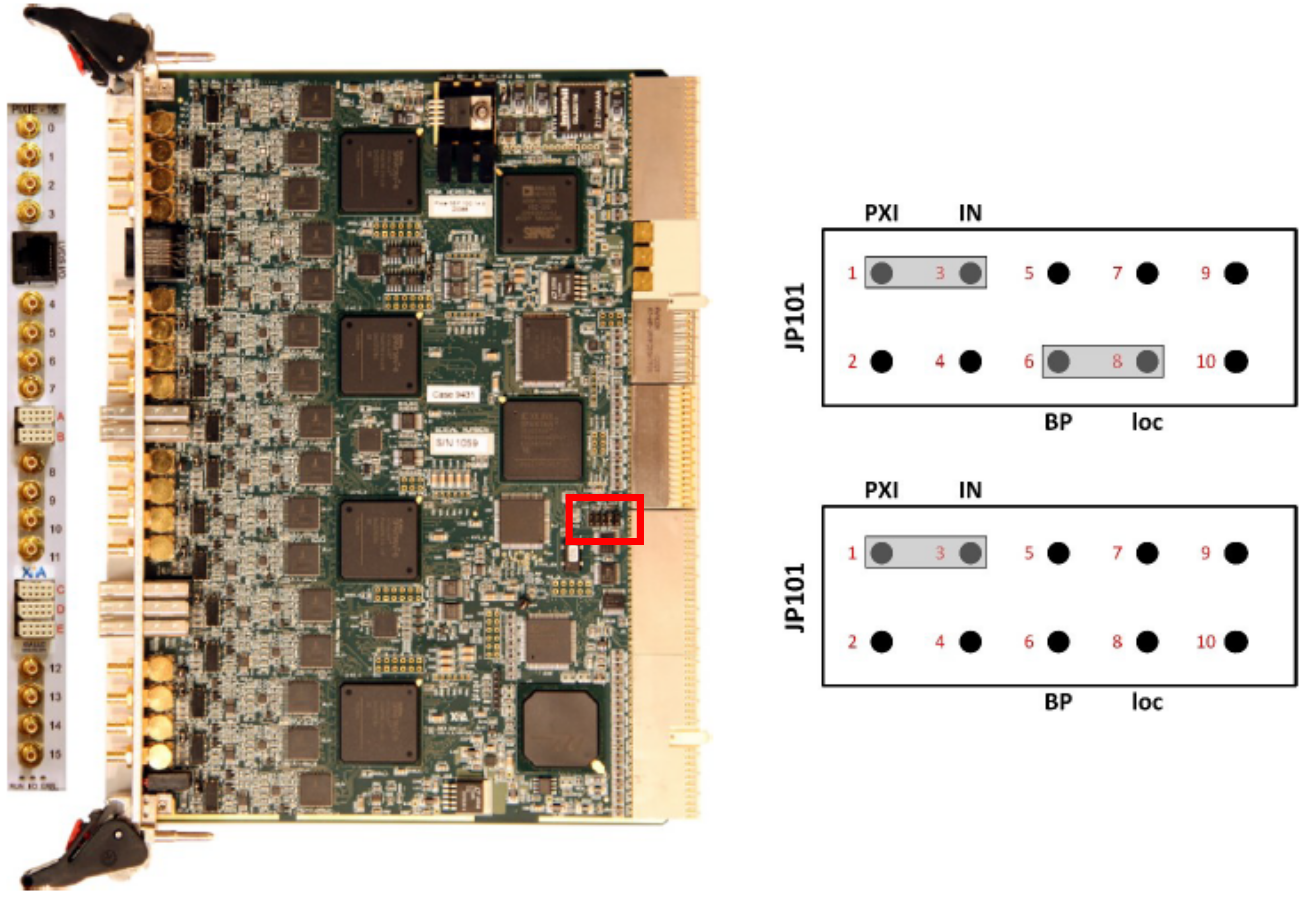
[Left] A Pixie-16 board with the location of the JP01 jumper block shown in the red box. [Right] Schematic of the jumper settings for distributing the clock across the PXI backplane for a single-crate system. Top: PXI clock master jumper settings (slot 2). Bottom: PXI clock recipient jumper settings (slots 3-14). Figures reprinted from 'Pixie-16 User Manual', Version 3.06, XIA LLC.

: In this configuration your clock-master module must be installed in slot 2. If more modules are added to the system, their jumper configuration should match the configuration shown on the bottom right of the above figure.

Configuring an Input Signal

: A test signal from a pulser is used for this tutorial. Setup the pulser to output pulses that rise quickly but have an approximately 50 μs decay time. The test pulse should be negative (-) polarity, have an input voltage of less than 1 V and a frequency less than 5 kHz. Connect the test signal to channel 0 of the digitizer.

Example Configuration Files

: The setup described in this tutorial uses a single digitizer installed in slot 2 of the PXI crate. Our DSP settings are stored in the file crate_1.json in a readout directory on our development system. Our cfgPixie16.txt file looks like:

1  # crateID
1  # number of modules
2  # slot for mod 0
/user/0400x/ddas_xiatest/readout/crate_1/crate_1.json

: The modevtlen.txt file must consist of (at least) a single line specifying that there are 4 expected data words (no optional settings are enabled).

Configuring DSP Settings Using QtScope

Once you have a correctly configured working directory, it is time to program the module with appropriate settings for the test signal. The QtScope program is used to view input waveforms and set DSP parameters. QtScope is installed as part of the NSCLDAQ software package and should be run by:

source /usr/opt/daq/12.1-xiaapi4/daqsetup.bash.
$DAQBIN/qtscope

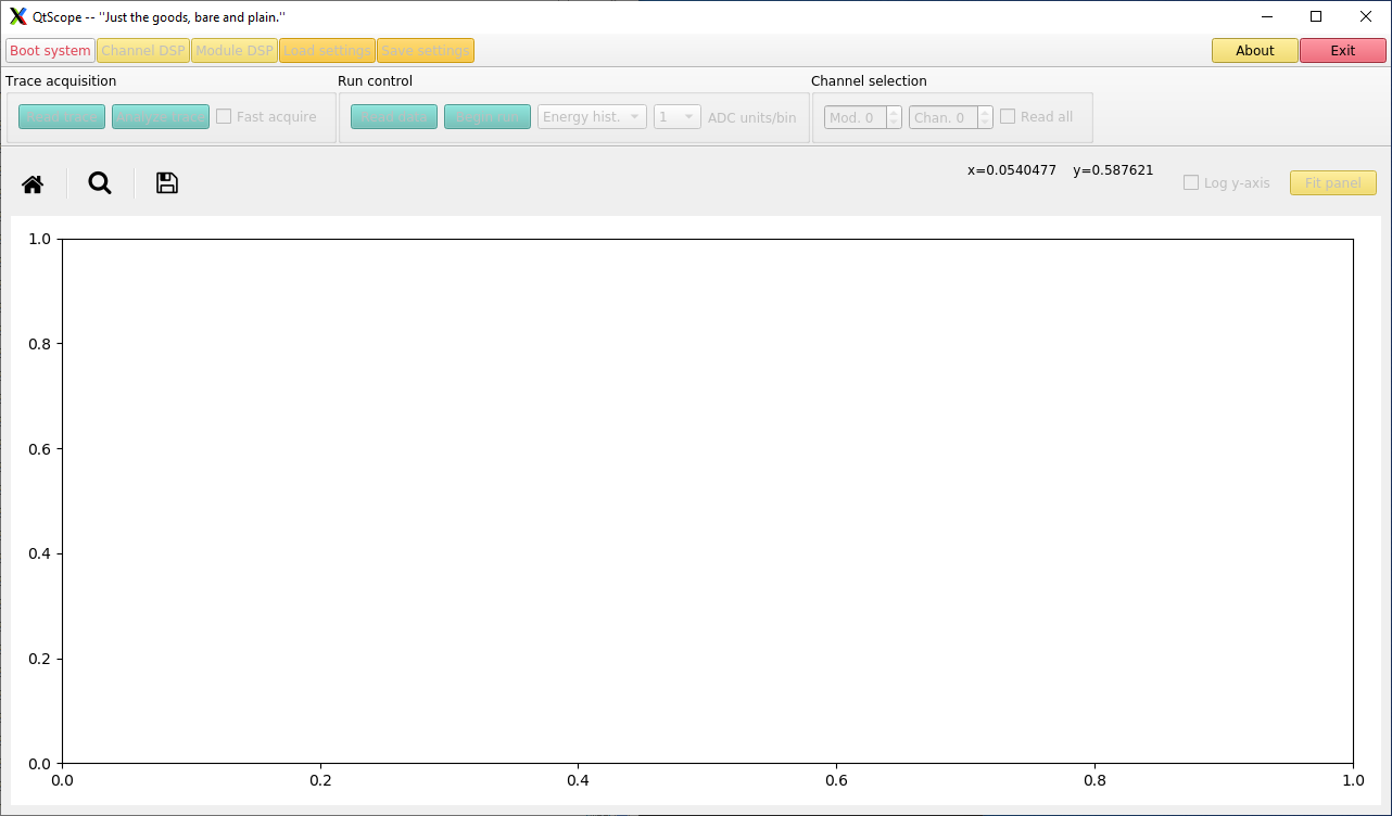
The QtScope GUI state on startup. Note that most GUI elements besides [Boot system], [About], and [Exit] on the system toolbar are disabled.

: The QtScope GUI will launch. See the QtScope documentation for more details, only the basics are covered in this guide. Most features of the GUI are inaccessible (grayed out) until the modules have been booted. To boot the modules, click the [Boot system] button. QtScope will print some information on the terminal where it was launched. A successful boot will look something like:

------------------------
Initializing PXI access...
System initialized successfully.
Found Pixie-16 module #0, Rev = 15, S/N = 1150, Bits = 16, MSPS = 250

Booting Pixie-16 module #0
        ComFPGAConfigFile:  /usr/opt/ddas/firmware/2.2-000/firmware/syspixie16_current_16b250m.bin
        SPFPGAConfigFile:   /usr/opt/ddas/firmware/2.2-000/firmware/fippixie16_current_16b250m.bin
        DSPCodeFile:        /usr/opt/ddas/firmware/2.2-000/dsp/Pixie16_current_16b250m.ldr
        DSPVarFile:         /usr/opt/ddas/firmware/2.2-000/dsp/Pixie16_current_16b250m.var
        DSPParFile:         /user/0400x/ddas_xiatest/readout/crate_1/crate_1.json
------------------------------------------------------

All modules ok
QtScope system configuration complete!

: If the boot fails, detailed error messages are written to Pixie16Msg.log and qtscope.log. Looking at the information contained in these log files should provide some context for the boot error and may point to a solution.

Analog Signal Conditioning

: The first thing we must do is setup the ADC for our input signal. First, lets look at a trace. Click the [Read trace] button until you see a full waveform trace. Here is an example trace:

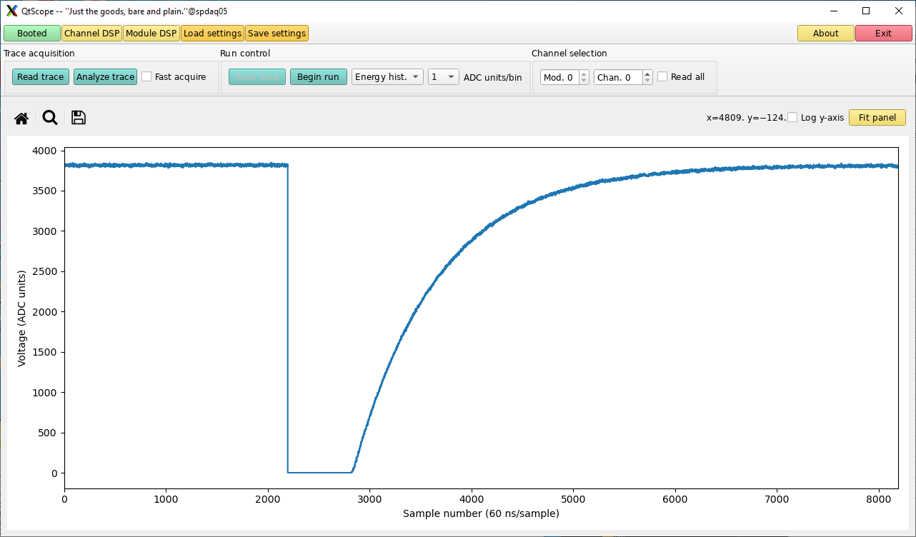
A raw pulser trace captured by QtScope. The DSP settings have not been properly configured for the test pulse, see the text for details.

No matter the input signal polarity, the QtScope canvas should display a positive-polarity signal. Knowing that, two things immediately jump out about the above example:

The displayed signal polarity is wrong. This is an indication that a negative-polarity signal is assumed to be positive by the Pixie DSP FPGA.
The signal is clipped. That is, the pulse is out of range of the ADC, in this case, extending below 0.

: In order to correct these issues we need to configure some channel DSP settings on the module. Clicking on the [Channel DSP] button will open a popup menu that looks like:

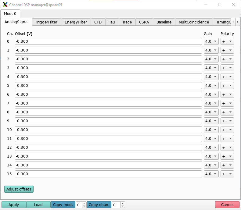
The QtScope analog signal conditioning tab.

: Our pulser test signal is plugged in to channel 0. Using the combo box in the polarity column, select negative (-) polarity for channel 0. Click the [Apply] button at the bottom of the channel DSP window to program the module with the new settings. Our analog signal tab now looks like:

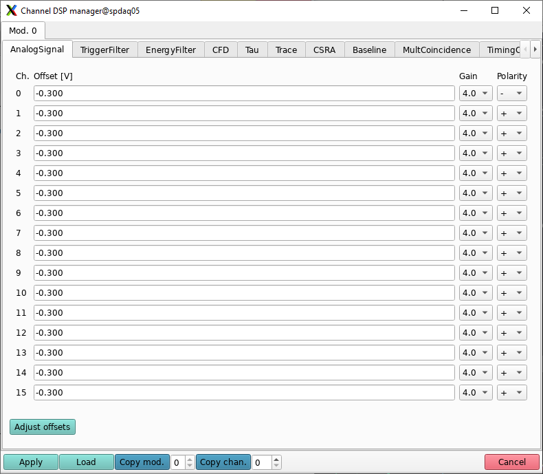
The QtScope analog signal conditioning tab with the polarity on channel 0 set correctly for our negative-polarity test signal.

: If we acquire another trace with these settings, we see:

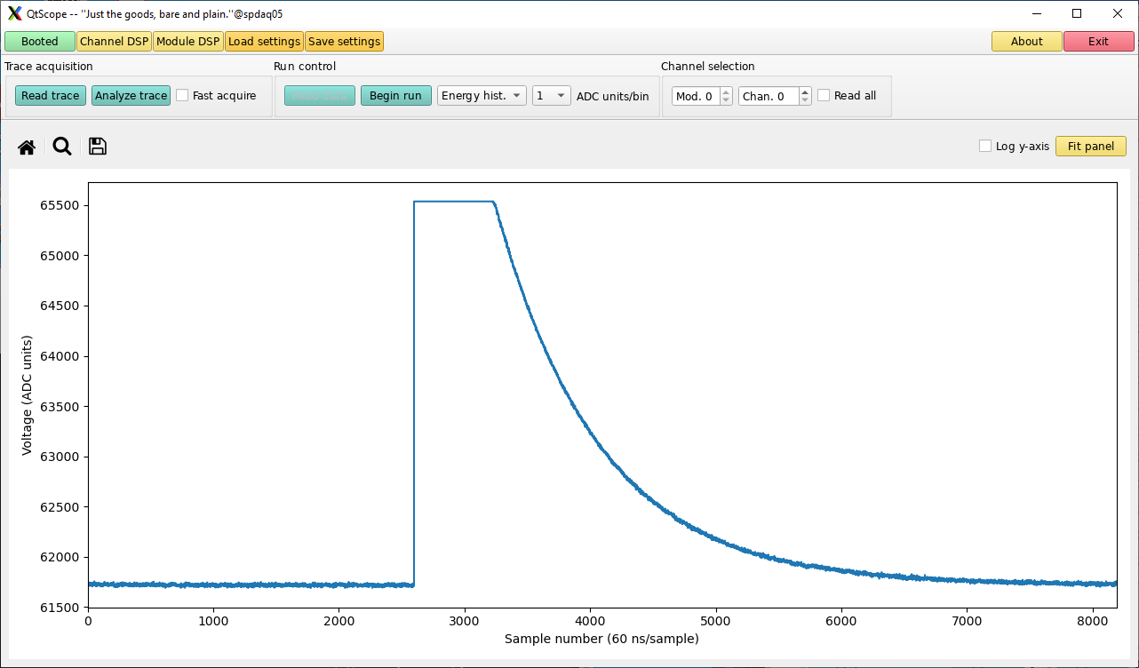
A raw pulser trace captured by QtScope. The pulse polarity has been set correctly (the pulse is displayed with positive polarity), but the waveform is still clipped and overflows the ADC.

: While the signal polarity has been configured correctly, the trace is still clipped, this time at the top of the ADC range. The DC offset must be adjusted such that the digitized signal falls within the voltage range of the ADC. Fortunately, the Pixie modules have a way of determining this offset automatically. Click the [Channel DSP] button to again bring up the channel DSP manager popup window. Clicking the [Adjust offsets] button on the AnalogSignal tab will prompt the module to automatically determine good DC offset values. By default, the DC offset will be automatically set such that the signal baseline sits at approximately 10% of the full ADC range. Do not forget to click the [Apply] button after adjusting the offsets!

The QtScope analog signal conditioning tab after automatic adjustment of the DC offset values.

: Reading another waveform gives the expected signal:

A raw pulser trace captured by QtScope with correctly configured polarity and DC offset. The full pulse is within the voltage range of the ADC.

Configuring the Trigger Filter

: Next we will configure the trigger settings for our test signal. Open the channel DSP manager window and select the TriggerFilter tab. This tab contains the DSP settings which parameterize the trapezoidal filter used to construct a leading-edge trigger for the input signal. An in-depth discussion of trapezoidal filters and other pulse-processing methods are beyond the scope of this guide; for more information refer to Further Reading.

: Our test signal has a fixed amplitude and pulse shape and very little noise. Note that in general only some (or none!) of these things may be true. We will use a triangular filter with a risetime of 100 ns and a gap of 0 ns. The triangular filter is simply a special case of a trapezoidal filter with a gap equal to 0. The value of the trigger threshold must be set such that we can trigger on the input test pulse; because we have a fixed-height pulse, there is not much to do here: We set the trigger to have a risetime of 100 ns, gap of 0 ns, and a threshold of 50. Once the settings are applied, note that the channel DSP GUI reports a trigger risetime of 104 ns: the filter parameter values must be an integer number of FPGA clock cycles and are automatically rounded to a valid value if they are not. Because the 250 MSPS modules use a 125 MHz FPGA, the filter lengths must be an integer multiple of 8 ns.

The trigger filter settings for our test pulse. A triangular filter (gap = 0 ns) is used. Note that the risetime and gap of the filter must be integer multiples of the signal-processing FPGA clock cycle which is equal to 10 ns for 100 MSPS and 500 MSPS modules and 8 ns for 250 MSPS modules.

Note: In a production setup, the trigger threshold should typically be set as low as possible without triggering on noise and is detector- and environment-specific.

Configuring the Energy Filter and Pole-Zero Correction

: Next we will configure the settings necessary to generate a good energy spectrum from our test pulse. We should expect to see a high-resolution Gaussian energy response without any background. Make sure that the Channel Selection Box is set to display results from the channel the test signal is plugged into and that the "Read all" option is disabled. Start a histogram run by ensuring that "Energy hist." is displayed in the drop-down menu in the Run Control Box of the Acquisition Toolbar and clicking [Begin run]. You should see the text

Beginning histogram run in Mod. 0

: appear in the terminal window you used to launch QtScope. Click the [Read data] button a few times to read data into the histogram. If the DSP are set improperly, you might see the following:

An energy spectrum for our test pulse acquired with bad energy DSP settings. The response is not Gaussian and is much broader than one would expect from a pulser signal.

: Click the [End run] button to stop taking data. When the run is ended, an end-of-run message and run statistics are printed to the terminal where QtScope is running:

Ended histogram run in Mod. 0
Module 0 channel 0 input 1503.21 output 1503.21 livetime 48.5719 runtime 48.5719
Module 0 channel 1 input 0 output 0 livetime 48.5719 runtime 48.5719
Module 0 channel 2 input 0 output 0 livetime 48.5719 runtime 48.5719
Module 0 channel 3 input 0 output 0 livetime 48.5719 runtime 48.5719
Module 0 channel 4 input 0 output 0 livetime 48.5719 runtime 48.5719
Module 0 channel 5 input 0 output 0 livetime 48.5719 runtime 48.5719
Module 0 channel 6 input 0 output 0 livetime 48.5719 runtime 48.5719
Module 0 channel 7 input 0 output 0 livetime 48.5719 runtime 48.5719
Module 0 channel 8 input 0 output 0 livetime 48.5719 runtime 48.5719
Module 0 channel 9 input 0 output 0 livetime 48.5719 runtime 48.5719
Module 0 channel 10 input 0 output 0 livetime 48.5719 runtime 48.5719
Module 0 channel 11 input 0 output 0 livetime 48.5719 runtime 48.5719
Module 0 channel 12 input 0 output 0 livetime 48.5719 runtime 48.5719
Module 0 channel 13 input 0 output 0 livetime 48.5719 runtime 48.5719
Module 0 channel 14 input 0 output 0 livetime 48.5719 runtime 48.5719
Module 0 channel 15 input 0 output 0 livetime 48.5719 runtime 48.5719

: where the input and output count rates give the rates of seen and accepted triggers (in triggers per second). The livetime and realtime count the amount of time (in seconds) the system was live and the total length of the run. System deadtime is calculable from these values: deadtime = (1 - livetime)/realtime.

: The energy response for our test signal is clearly non-Gaussian and has a resolution of approximately 1.8% FWHM. This is an indication that the DSP settings which govern the energy response are not set correctly. Four DSP parameters govern the energy response: the energy filter risetime, gap, and filter range which parameterize the trapezoidal filter used to determine the energy, and the tau parameter which sets the pole-zero correction for the filter output.

: The filter range parameter controls how many samples are averaged together prior to the energy filtering logic. In general this value should be set to the smallest value which can accommodate the filter length you want to use. The energy filter risetime and gap again parameterize the trapezoidal filter. The gap, which cannot be 0 for the energy filter, should be set to a value longer than the longest-expected risetime from your input signal. Optimizing the risetime depends on the particular properties of the signal, expected rate, desired resolution, etc., which depend on your particular system. The tau parameter should be set to the decay time constant of the input signal (for example, from a preamplifier).

: For our test signal, a risetime of 600 ns, gap of 256 ns and tau of 50 μs are reasonable initial guesses based on how we configured the signal from the pulser:

The EnergyFilter [left] and Tau [right] DSP settings used for our test signal in channel 0.

: Once applied, a new energy spectrum is acquired:

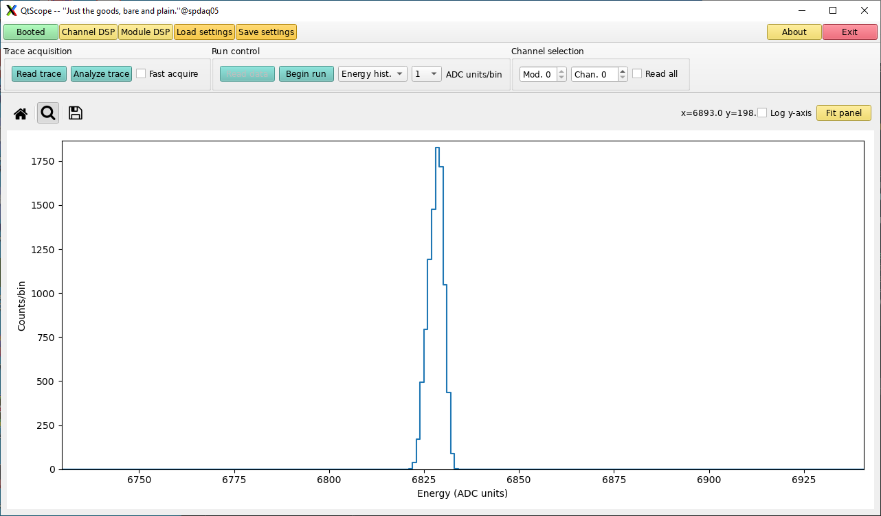
An energy spectrum for our test pulse acquired with good energy DSP settings. Note the Gaussian-like signal shape and improved energy resolution compared to the previous settings.

: The peak more closely resembles the expected Gaussian shape, and the energy resolution is improved to approximately 0.2% FWHM. Further optimizations to the resolution and signal shape may be possible by varying the aforementioned parameters; this manner of detailed optimization is left as an exercise for the reader.

Save Your Updated Settings

: Once your test channel DSP is set to your satisfaction, save your settings by clicking the [Save settings] button. Enter a file name and click the "Save" button. Make sure to update your cfgPixie16.txt file so that it points to your updated settings file if needed!

Taking Data With DDASReadout

Now that you have a good settings file, you can take data using a readout program. In this section we will:

Run DDASReadout, the module readout code for DDAS,
Run the NSCLDAQ dumper program to look at raw event data,
Take a bit of data and describe its format.

: Full documentation for the readout program is available here.

: The DDAS readout programs do not need to be modified. They use a set of configuration files that are expected to live in the current working directory when readout is run. These files were discussed in Configuration Files Needed by NSCL DDAS. In the previous step you should have generated a new settings file and edited your cfgPixie16.txt file if necessary. The modevtlen.txt file must be edited to reflect the size of the events we expect coming from each module. We are using only a single module and not taking waveforms or any other additional data from that module. Since the modevtlen.txt file format is simply the size of an event, in 32-bit words, from each digitizer's channels, one digitizer per line, in the same order as the cfgPixie16.txt file, the contents of this file should be:

: which is the default Pixie channel data length in 32-bit words. Now that the configuration files are correct, you can run the readout program. Remember that at FRIB the NSCLDAQ software is intended to be run under a container image! Here we assume that your readout directory is ~/readout/crate_1:

cd ~/readout/crate_1

$DAQBIN/DDASReadout

: Running this command will boot the modules in the crate. If the boot is successful you should see some output indicating it is ready:

...
The new event buffer size will be: 16934
Using a FIFO threshold of 10240 words
Trying to initialize Pixie
Crate number 1: 1 modules, in slots:2 DSPParFile: /user/0400x/ddas_xiatest/readout/crate_1/crate_1.json
Module event lengths: 4
------------------------
Initializing PXI access...
System initialized successfully.
Found Pixie-16 module #0, Rev = 15, S/N = 1150, Bits = 16, MSPS = 250

Booting Pixie-16 module #0
        ComFPGAConfigFile:  /usr/opt/ddas/firmware/2.2-000/firmware/syspixie16_current_16b250m.bin
        SPFPGAConfigFile:   /usr/opt/ddas/firmware/2.2-000/firmware/fippixie16_current_16b250m.bin
        DSPCodeFile:        /usr/opt/ddas/firmware/2.2-000/dsp/Pixie16_current_16b250m.ldr
        DSPVarFile:         /usr/opt/ddas/firmware/2.2-000/dsp/Pixie16_current_16b250m.var
        DSPParFile:         /user/0400x/ddas_xiatest/readout/crate_1/crate_1.json
------------------------------------------------------

All modules ok
Module #0: module ID word=0xf1000fa, clock calibration = 8
Setup scalers for 1 modules
Scalers know crate ID = 1
%

: The information displayed here should reflect the physical hardware installed in your crate and match the slot map, settings file, and event lengths that you specified in the cfgPixie16.txt and modevtlen.txt configuration files. The program will wait in this ready state until it is told to begin taking data.

Starting the NSCLDAQ dumper Program

: Open a new terminal window and run the dumper program by typing

$DAQBIN/dumper --count=50

: on the command line. Note that this requires you to source the daqsetup.bash script and must be run under the container as described previously. The dumper program allows us to examine data in the ringbuffers and is a powerful tool for low-level debugging. The --count=50 option will cause the dumper to dump 50 events then exit.

Taking Data and Looking at the Format

: Start taking data with DDASReadout by switching back to the window where it is running. Type begin at the command prompt (the % character). The dumper window should output a lot of text and the dumper should exit back to the shell. Once the dumper exits you can stop data taking by typing end in the terminal window where the DDASReadout program is running. Typing exit will close the readout program.

: Lets take a closer look at the dumped event data. The actual contents of the event we analyze may be different from what you see in your test, we are only interested in explaining the structure of the event at this time.

...
-----------------------------------------------------------
Event 16416 bytes long
No body header
2010 0000 00fa 0f10 0000 0000 0000 4020 
4020 0008 a9b2 39d8 0000 390f 0140 0000 
4020 0008 0691 39d9 0000 394c 0147 0000 
4020 0008 6370 39d9 0000 3c10 013f 0000 
... many more events ...

: This data comes from the first step of the full readout pipeline we will discuss in more detail as we progress in the tutorial. It contains some identifying information about the data and where it comes from followed by a collection of hits from that module. These hits may or may not be time-ordered. The first line contains identifying information about the module. Each line after the first contains 4 32-bit words of Pixie data as specified in the modevtlen.txt file.

: The first two words of the event body 2010 0000 are the self-inclusive event size in 16-bit words, given in little endian format. This means that the first word is the least significant part while the second word is the most significant part. The event size is 8208 16-bit words (we are only showing part of the event above). Data from the digitizer comes in 32-bit longwords. Therefore each pair of values is a digitizer longword.

: Looking at the first two lines will help us understand the data format. The words and their meaning are:

Data word	Meaning
`0x00002010` (32 bits)	Self-inclusive event size in 16-bit words.
`0x0f1000fa` (32 bits)	Module identifier (ADC bits, board revision, module MSPS)
`0x4020000000000000` (64 bits)	Module clock calibration in nanoseconds. A 64-bit double in IEEE 754 format.
`0x00084020` (32 bits)	Pixie event header word 0: event and channel ID.
`0x39d8a9b2` (32 bits)	Pixie event header word 1: low-order timestamp.
`0x390f0000` (32 bits)	Pixie event header word 2: high-order timestamp (lower 16 bits) and CFD interpolation (upper 16 bits).
`0x00000140` (32 bits)	Pixie event header word 3: energy (lower 16 bits) and trace info (upper 16 bits)

: The event has a 48-bit timestamp which is constructed by combining the low-order timestamp contained in word 1 with the high-order timestamp contained in the lower 16 bits of word 2. The timestamp given in the raw data is in FPGA clock ticks. The module clock calibration written in the third word of the event data allows us to convert this timestamp into nanoseconds allowing us to compare and correlate events coming from a heterogeneous set of digitizers in the system. As you can see, the Pixie event header structure repeats on every line after the first.

Running ddasReadout Using the ReadoutGUI

: This section describes how to configure data sources, setup an event builder and run the readout driver for DDAS in a "production-like" mode using the ReadoutGUI. For users familiar with previous versions of FRIBDAQ software, the data-source configuration is done slightly differently in FRIBDAQ 12, reflecting the fact that the module readout and timestamp ordering processes are separated. The ddasReadout program allows us to run the module readout and timestamp sorting as if it were a single process.

Setting up SSH keys for Password-Less Login

: ReadoutGUI is built to allow you to run your experiment software distributed across several systems. To do this, it runs your readout program on the end of an SSH pipeline. Normally, starting SSH requires that you provide a password to the account it logs into on the remote (or local) system. In this section we will describe how to avoid the need to provide a password every time ReadoutGUI starts up an SSH session. The process hinges on SSH's ability to not only use passwords to authenticate but also to use an asymmetric certificate, or key, to identify and authenticate a login.

In this section we'll go through the procedure to create and install what are called the private and public keys. Once installed, these allow you to SSH to your account in any system that shared your home directory without providing a password. This process requires that you:

Create public and private ssh keys.
Install your public key into your authorized keys file
Ensure that directory permissions are set up to SSH's satisfaction.

: To create public and private key files, use ssh-keygen:

0400x@spdaq05:~$ ssh-keygen -t rsa
Generating public/private rsa key pair.
Enter file in which to save the key (/home/a/.ssh/id_rsa): 
Created directory '/home/a/.ssh'.
Enter passphrase (empty for no passphrase): 
Enter same passphrase again: 
Your identification has been saved in /home/a/.ssh/id_rsa.
Your public key has been saved in /home/a/.ssh/id_rsa.pub.
The key fingerprint is:
3e:4f:05:79:3a:9f:96:7c:3b:ad:e9:58:37:bc:37:e4

: Note that we will use an empty passphrase in the dialog above. Otherwise SSH will prompt us for the passphrase prior to using the keys, which leaves us no better off than before. ssh-keygen will generate a pair of files: ~/.ssh/id_rsa and ~/.ssh/id_rsa.pub. id_rsa.pub must be added to ~/.ssh/authorized_keys:

cat ~/.ssh/id_rsa.pub >> ~/.ssh/authorized_keys

We're almost there. SSH wants to secure your account so that:

Your private key, ~/.ssh/id_rsa cannot be stolen and
Nobody can implant additional keys into ~/.ssh/authorized_keys.

chmod g-w,o-w ~
chmod 0700 ~/.ssh
chmod 0600 ~/.ssh/id_rsa
chmod 0600 ~/.ssh/authorized_keys

: Finally test this at FRIB:

ssh nucleus

: If you've followed this procedure properly, you should login to a nucleus system without being asked to give a password. We're going to set up the ReadoutShell so that it will later run the ReadoutGUI with the NSCL Event builder. While strictly speaking, the event builder is not needed for a single module, normally it is used. This makes the final event structure uniform.

Stage Areas and Recording Data

: In addition to running the readout driver program, ReadoutGUI can initiate data recording. To do this, ReadoutGUI must be told where to record data. ReadoutGUI expects a symbolic link in your home directory named stagearea. This link points to a directory structure into which event data are logged. For more information about the directory structure ReadoutGUI maintains, see the NSCLDAQ user guide section on the ReadoutGUI found here.

Setting Up the Data Sources

: First we will setup the ddasReadout program as a data source. Data sources are programs that are managed by the ReadoutGUI and create data. We're going to use the convention that readout programs will produce raw data into rings named username_raw_n where n is the crate number. In our example, the user is 0400x, so our raw ring name will be 0400x_raw_1. The readout driver also manages a sorter. Data is read from the raw ring, sorted by timestamp, and output into a sorted ringbuffer. We will use the convention of username_sort_n for the sort ring, i.e. 0400x_sort_1. At present, ReadoutGUI is not aware of environment variables. Thus you need to determine what DAQBIN means when setting up your data sources. For this example, we'll assume it translates to /usr/opt/daq/12.1-xiaapi4/bin.

: Start the ReadoutShell:

$DAQBIN/ReadoutShell

: This command opens the ReadoutShell GUI window:

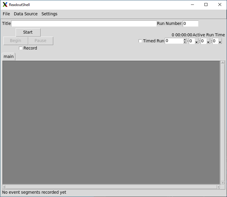
The ReadoutShell GUI window. The GUI allows users to configure data sources and run the DAQ from a single interface.

Once the GUI is open,

Use the Data Source->Add... menu entry to add a new data source.
From the data source type dialog select SSHPipe from the list of data source types and click Ok.

: This should bring up the following window:

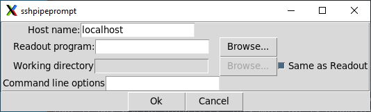
The SSHPipe data source configuration prompt. The fields in this interface are used to configure the DDAS data sources for our experiment.

: In the resulting dialog, fill in the fields as follows:

Field name	Contents
Host name:	Name of the host on which the readout will run. I used: spdaq05.
Readout program:	The readout driver program from your `$DAQBIN`. Enter the full path or navigate to that directory using the `Browse` button. I used: /usr/opt/daq/12.1-xiaapi4/bin/ddasReadout.
Working directory	Set to the directory containing the DDAS configuration files. Un-check the "Same as Readout" box and either enter the full path or navigate to that directory using the `Browse` button. I used: /usr/0400x/ddas_xiatest/readout/crate_1
Command line options	Options for running the readout driver code. I used: -readouthost spdaq05 -readoutring 0400x_raw_1 -sorthost spdaq05 -sortring 0400x_sort_1 -cratedir /user/0400x/ddas_xiatest/readout/crate_1

: Click the Start button to start your data source. A new tab should pop up on the ReadoutGUI for your SSHPipe data source. This tab is used to capture and display messages on stdout and stderr for the readout driver. If you select this tab you should see, among other things, the same boot information you have seen previously in Taking Data With DDASReadout.

: Let's check that this all works. You can run the dumper as follows:

$DAQBIN/dumper --source=tcp://spdaq05/0400x_raw_1 --count=50

: to dump 50 items from the raw ring. Start a run by clicking the Begin button on the ReadoutGUI. Make sure that there is data being emitted by the dumper. This data should look like the data we discussed in the previous section. You can also look at the sort ring data:

$DAQBIN/dumper --source=tcp://spdaq05/0400x_sort_1 --count=50

: The events in the sort ring look like:

-----------------------------------------------------------
Event 24 bytes long
Body Header:
Timestamp:    9416064
SourceID:     0
Barrier Type: 0
000c 0000 00fa 0f10 4020 0008 f5b0 0011 
0000 68f1 0142 0000

There are three big differences between the sort ring data and the raw ring data:

The events in the ringbuffer are time-ordered.
Each event contains only data from one channel.
There is an event header containing, among other things, the event timestamp in nanoseconds.

: The first two 32-bit words are the same as described previously: the self-inclusive event size and the module identification word. The next 4 words are the Pixie event header data. Note that the full 48-bit timestamp 0x00000011f5b0 is equal to 1177008 clock ticks. Multiplying this number by 8 ns/clock tick for the 250 MSPS module gives the timestamp 9416064 displayed in the event header. The output of the sort ring is used as the input to the event builder, which we will discuss in the following section.

Setting Up the Event Builder

The event builder is used to create a single, ordered, merged data stream from an arbitrary number of clients (data sources). While strictly speaking, the event builder is not needed for a single module, normally it is used. This helps enforce some uniformity in the final event structure. Starting the event builder is a matter of creating a ReadoutCallouts.tcl script which

Incorporates the event builder API into the ReadoutGUI
Adds an OnStart proc (the Tcl equivalent to a function in other languages) that configures and starts the event builder.
Register a ring source as a feeder process from our sorted data ring (0400x_sort_1) to the event builder.

: Here is an example of a ReadoutCallouts.tcl script that does this for our case:

package require evbcallouts                                                             (1)

::EVBC::useEventBuilder                                                                 (2)

proc OnStart {} {
    ::EVBC::initialize -restart true -glombuild true -glomdt 100 -destring 0400x_evb    (3)
}

::EVBC::registerRingSource tcp://spdaq05/0400x_sort_1 "" 0 Crate_1_DDAS 1 1 5 0         (4)

This line incorporates the event builder API into the ReadoutGUI.
::EVBC::useEventBuilder installs the event builder state change handlers into the ReadoutGUI. The state change handlers allow the event builder API to take actions when the run state changes.
::EVBC::initialize starts the event builder. The parameter you'll want to adjust is -glomdt, which specifies the event builder's coincidence window. Generally speaking, the units for this value are the same as the units of the timestamp. If you are only dealing with a single DDAS readout program, your coincidence window will be in units of nanoseconds, because the timestamps are converted to units of nanoseconds prior to being outputted from the readout program.
::EVBC::registerRingSource adds a ring data source to be started at the beginning of a run. This is a feeder from a ringbuffer to an event builder that runs in the localhost. The parameters are, in order: the source ringbuffer URL; the timestamp extraction library (which can be empty); the source id (which must be the same as the --sourceid parameter for the readout); a comment that will be displayed in the event builder GUI; a flag that, if 1 indicates that the data will have timestamps in body headers (no timestamp extractor is needed); a flag which, if true means the source will exit when it sees an end of run; a timeout, in seconds, to wait after the source has observed an end run item; a time offset which is added to the timestamp to compensate for synchronization effects. Spaces in the comment must be escaped using the \ character.

: If we restart the ReadoutShell, begin a run, and point the dumper at the data in 0400x_evb we can take a look at the format of a built event. This one is typical:

-----------------------------------------------------------
Event 76 bytes long
Body Header:
Timestamp:    9394456
SourceID:     0
Barrier Type: 0
004c 0000 5918 008f 0000 0000 0000 0000 
0034 0000 0000 0000 0034 0000 001e 0000 
0014 0000 5918 008f 0000 0000 0000 0000 
0000 0000 000c 0000 00fa 0f10 4020 0008 
eb23 0011 0000 3aa4 0142 0000

: Let's pick apart the data for this event. Note that it is much bigger than the sort ring events. This is because the data are framed with a fragment header which also encapsulates a ring item header that in turn wraps the event body. To get on familiar territory, note that in the last lines:

000c 0000 00fa 0f10 4020 0008 eb23 0011
0000 3aa4 0142 0000

: we see the same raw data as before: the event size, module ID word, and Pixie data header. We're going to pick apart the data prior to this, much of which is only relevant if you are using multiple crates. Here is the short summary of the information prior to the raw event. First is the fragment header:

Data word	Meaning
`0x0000004c` (32 bits)	Total event size in bytes.
`0x00000000008f5918` (64 bits)	Event builder fragment timestamp in nanoseconds. This is 8x the digitizer timestamp for our 250 MSPS module.
`0x00000000` (32 bits)	Data source ID (value of `--sourceid` for the readout).
`0x00000034` (32 bits)	Size of the fragment payload in bytes (not self-inclusive)
`0x00000000` (32 bits)	Barrier type.

: Next are the ring item and ring item body headers:

Data word	Meaning
`0x00000034` (32 bits)	Number of bytes in the ring item (self-inclusive).
`0x0000001e` (32 bits)	Ring item type (PHYSICS_EVENT).
`0x00000014` (32 bits)	Number of bytes in the body header. The body header contains information used by the event builder.
`0x00000000008f5918` (64 bits)	Fragment timestamp in nanoseconds.
`0x00000000` (32 bits)	Fragment source ID.
`0x00000000` (32 bits)	Fragment barrier type.
`0x0000000c` (32 bits)	First word of the fragment.

: if several fragments got glued together to create a single event (as will happen if you tee off your pulser into several channels), there will be a ring item in the fragment body for each fragment that made the coincidence requirement.

Analyzing Data With SpecTcl

: SpecTcl is the lab-supported framework for analyzing data online. DDAS comes with some tools to use in unpacking DDAS data within the context of SpecTcl, DAQ::DDAS::DDASUnpacker and DAQ::DDAS::DDASBuiltUnpacker. These both provide support for parsing the raw data of DDAS for you. It is in your best interest to leverage these tools rather than writing your own unpacker. To learn how to use the DAQ::DDAS::DDASBuiltUnpacker in your SpecTcl, please refer to Analyzing DDAS Data in SpecTcl.

Conclusions

: This concludes the single-crate setup tutorial. You should now have a good understanding of how to perform the basic steps necessary to configure a simple DDAS system to take data. The modules have many features which are not discussed in detail in this section, including a digital CFD for precision timing, the ability to run complex coincidence triggers, or take additional data such as QDC sums or, more commonly, ADC trace data. Refer to the QtScope Manual for more information.

Appendix A: Data Format

: This section describes the bit fields present in words of a DDAS event. This information is supplemental to the description provided in Taking Data and Looking at the Format. Values in the table below refer to the first and second lines of the following event:

...
-----------------------------------------------------------
Event 16416 bytes long
No body header
2010 0000 00fa 0f10 0000 0000 0000 4020 
4020 0008 a9b2 39d8 0000 390f 0140 0000 
4020 0008 0691 39d9 0000 394c 0147 0000 
4020 0008 6370 39d9 0000 3c10 013f 0000 
... many more events ...

The module identification word 0x0f1000fa has the following fields:

Bits	Meaning	Value
0-15	Sampling frequency in MSPS	0xfa = 250
16-23	ADC bit depth of the digitizer	0x10 = 16
24-31	Module board revision number	0x0f = 15

: The key values from this word are that the digitizer runs at 250 MSPS and captures waveforms with 16-bit precision. The event header has several bit fields which are described in detail in the Pixie manual.

: The next data word in the event, 0x4020000000000000, stores the module clock calibration in nanoseconds per clock tick as an IEEE 754 double-precision value. A description of this format can be found online in many places including Wikipedia. The 250 MSPS modules use a 125 MHz clock for timestamping, so the clock calibration value is 8.0 nanoseconds per clock tick. Converting this value to IEEE 754 double format is left as an exercise for the reader.

: The first word of the Pixie event header is the most complicated and has many bit fields. The table below describes these fields and the values they have in the above event:

Bits	Meaning	Value
0-3	Channel number	0
4-7	Slot number (>= 2)	2
8-11	Crate ID	0
12-16	Header length (32-bit words)	4
17-30	Pixie event length (32-bit words)	4
31	Finish code (1 if piled up)	0

: The (self-inclusive) header length and (self-inclusive) event length have the same value in this case because no additional data (QDC sums, trace data, etc.) is being written.

Note: The meaning of the CFD bits in the Pixie event header depends on the type of digitizer being used. It is generally not necessary for users to understand these differences, as the DAQ::DDAS::DDASHit class and its derived classes abstract these differences away from the user.

Table of Contents